Alexander Bass

Math Notes 2026

I enjoy tinkering with math. Unfortunately, I often forget the little things I discover. On this page you will find all the tidbits I found interesting enough to record.

I don't strive for academic perfection, however I also do not want to spread blatant errors. If you notice any errors in these notes, please email me.

See all math notes

On Newton’s Method

Single Page

Newton’s method allows finding the ‘root’ of a function (where it is zero), given conditions expressed in the wikipedia article no doubt.

More than this however, it can be used to find the inverse of a function. The common example is 2\sqrt{2}. If you know xx where x22=0x^2-2=0, then you know 2\sqrt{2}.

The rough gist of the algorithm is as follows.

  1. Take a function like f(x)=x22f(x) = x^2-2
  2. Make an arbitrary guess on the value of xx where f(x)=0f(x)=0, g0g_0
  3. Evaluate f(x)f(x) at g0g_0 and find the line tangent to f(x)f(x) at g0g_0
  4. Find the x-intercept of the tangent line. This x-intercept value is g1g_1
  5. Repeat steps 2…5 (incrementing nn throughout) until a satisfactory precision is obtained.

Algebraically, we start with the function and its derivative:

f(x)=x22f(x)=2x \begin{aligned} f(x)&=x^2-2 & f'(x)&=2x \end{aligned}

And make a guess g0g_0 and create the tangent line at that guess location on f(x)f(x)

y=f(g0)x+b y = f'(g_0)x + b

find bb by evaluating at g0g_0:

f(g0)g0+b=f(g0) f'(g_0)g_0 + b = f(g_0) b=f(g0)f(g0)g0 b = f(g_0) - f'(g_0)g_0

Which finishes the line equation as:

y=f(g0)x+f(g0)f(g0)g0 y = f'(g_0)x + f(g_0) - f'(g_0)g_0

Next, find the x-coordinate by evaluating at y=0y=0

0=f(g0)x+f(g0)f(g0)g0f(g0)g0f(g0)=f(g0)xg0f(g0)f(g0)=x \begin{aligned} 0 &= f'(g_0)x + f(g_0) - f'(g_0)g_0\\ f'(g_0)g_0-f(g_0) &= f'(g_0)x\\ g_0 - \frac{f(g_0)}{f'(g_0)} &= x \end{aligned}

As stated above, this xx value is actually g1g_1, or generally

gn+1=gnf(gn)f(gn) g_{n+1} = g_n - \frac{f(g_n)}{f'(g_n)}

Going back the case of 2\sqrt{2}, we substitute in the function

gn+1=gngn222gn g_{n+1} = g_n - \frac{{g_n}^2-2}{2g_n}

With gn=5g_n=5 we see the first four approximations as:

g0=5g1=2.7g21.7204g31.4415g41.4145 \begin{array}{ccc} g_0 &= &5\\ g_1 &= &2.7\\ g_2 &\approx &1.7204\\ g_3 &\approx &1.4415\\ g_4 &\approx &1.4145\\ \end{array}

Generally…

This process is easily generalized to finding inverses instead of roots — just as in the 2\sqrt{2} example.

f(x)f(x) was previously defined as x22x^2-2, but more generically is described as f(x)=x2f(x)=x^2. Then, inside the recursive equation, the 2-2 is placed outside the function

gn+1=gnf(gn)2f(gn) g_{n+1} = g_n - \frac{f(g_n) - 2}{f'(g_n)}

The above gn+1g_{n+1} approximates f1(2)f^{-1}(2). the 22 is replaced with some constant cc to find f1(c)f^{-1}(c):

The generic case for c\sqrt{c} then is:

gn+1=gngn2c2gn g_{n+1} = g_{n} - \frac{{g_n}^2 -c}{2g_n}

Or

gn+1=gngn2c2gnlimngn=c \begin{aligned} g_{n+1} &= g_n - \frac{{g_n}^2-c}{2g_n}\\ \lim_{n \to \infty} {g_{n}} &= \sqrt{c} \end{aligned}

One way to loosely verify this is to: consider that when nn approaches \infty, the differences between gng_n and gn+1g_{n+1} will grow increasingly smaller (assuming the limit does indeed converge) and indeed will be come so close that we can consider them to be equal. So, we set gn+1=gn=xg_{n+1} = g_n = x and solve:

x=xx2c2xx2c2x=0x2=cx=c \begin{aligned} x &= x - \frac{x^2-c}{2x}\\ \frac{x^2-c}{2x} &= 0 \\ x^2 &= c\\ x &= \sqrt{c} \end{aligned}

Other inverses

This method can be extended to other functions. Some examples:

ln(x)gn+1=gn1+xegnlog2(x)gn+1=gn1+x2gnln(2)xgn+1=gngn+x \begin{array}{rcl} \ln(x) & \Rightarrow & g_{n+1} = g_n - 1 + \frac{x}{e^{g_n}} \\ \log_2(x) & \Rightarrow & g_{n+1} = g_n - 1 + \frac{x}{2^{g_n}\ln(2)} \\ x & \Rightarrow & g_{n+1} = g_n - g_n + x \end{array}

Approximate Functions

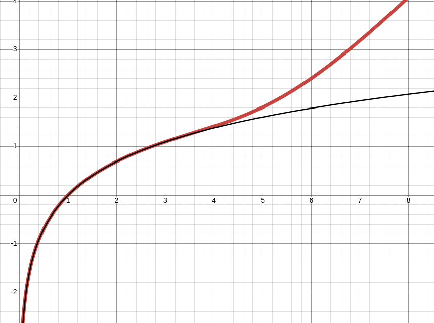
By expanding the recursion a few steps, we can create an obnoxious approximation for ln(x)\ln(x):

ln(x)xe1x+xexe1xx+2+xexe1xxexe1xx+2x+3+x4 \ln(x) \approx x e^{1 - x} + x e^{- x e^{1 - x} - x + 2} + x e^{- x e^{1 - x} - x e^{- x e^{1 - x} - x + 2} - x + 3} + x - 4

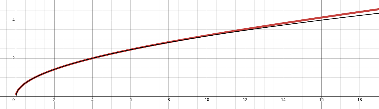
And one for x\sqrt{x}:

x0.0625x4+1.75x3+4.375x2+1.75x+0.06250.5x3+3.5x2+3.5x+0.5 \sqrt{x}\approx\frac{0.0625 x^{4} + 1.75 x^{3} + 4.375 x^{2} + 1.75 x + 0.0625}{0.5 x^{3} + 3.5 x^{2} + 3.5 x + 0.5}

In a way, this approximation for x\sqrt{x} is quite reasonably constructed. It has plenty of detail around the origin, but as it goes further the higher-order polynomial components divide out and all that is left is the slope asymptote.

These examples were generated with the Python library SymPy. (I got exhausted of writing it by hand around third recursion)

View Code
from sympy import symbols, simplify, print_latex

x = symbols("x")

expr = 1
for i in range(0, 3):
    expr = 0.5 * expr + x / (2 * expr)

print_latex(simplify(expr))

Newton’s Method Pi

Single Page

Suppose f(x)=sin(x)f(x)=\sin(x), then f(π)=0f(\pi) = 0. Using Newton’s method, we arrive at the recursion:

limngn=πwhereg0=3gn+1=gntan(gn) \begin{aligned} \lim_{n\to\infty} {g_n} &= \pi \\ &\text{where}\\ g_0 &= 3\\ g_{n+1} &= g_n - \tan(g_n) \end{aligned}

Which gives π accurate to 100 digits in only 5 iterations.

View Code
from sympy import N, tan, pi

expr = 3
for i in range(0, 5):
    expr = expr - tan(expr)

print(N(expr, 100))
print(N(pi - expr, 100))

The behavior of gn+1=gntan(gn)g_{n+1} = g_n - \tan(g_n) depends highly the initial value g0g_0. This makes some intuitive sense because sin(x)\sin(x) has many different roots so the sequence would likely converge to the nearest root to the starting point.

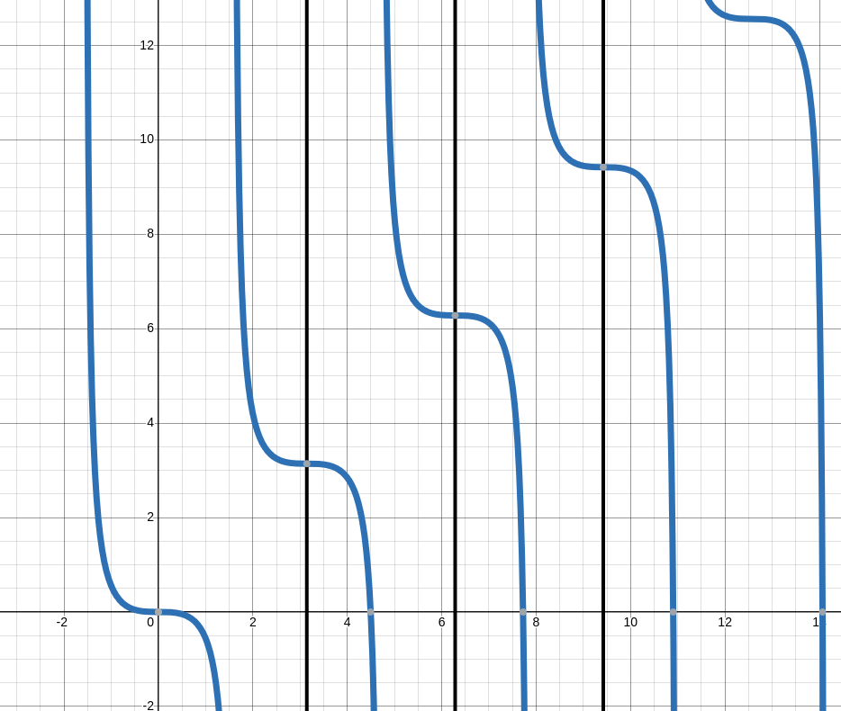
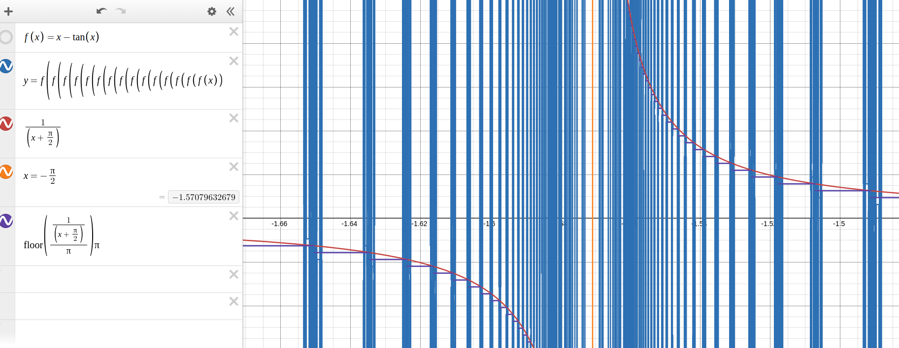
This behavior is clear by plotting f(x)=xtan(x)f(x) = x - \tan(x):

Around each multiple of pi, the graph flattens out. to the right of each flat point, the value of the function is decreases slightly. To the left, the value increases slightly. When the function is interpreted as the mapping from the previous value xx to the next value f(x)f(x), the slight decreases and increases near each multiple of π makes the recursion stably approach the nearest multiple of π. Further away from the multiples of π, the slope becomes steep enough to ‘push’ the next step of the recursion away from the nearest multiple of pi. The steep region is not well-behaved. for these notes, ‘well-behaved’ means that the recursion gn+1=gntan(gn)g_{n+1} = g_n - \tan(g_n) has a value which approaches the multiple of π nearest to g0g_0.

Specifically, let’s look at x=0πx=0\pi. The well-behaved region will extend an equal distance positive and negative from zero (because the function is symmetric to an extent around the multiples of π) Therefore, we can solve for this distance by finding gn=gn+1g_n = g_{n+1}, or x=(xtan(x))x=-(x-tan(x)).

2x=tan(x) 2x = \tan(x)

Or

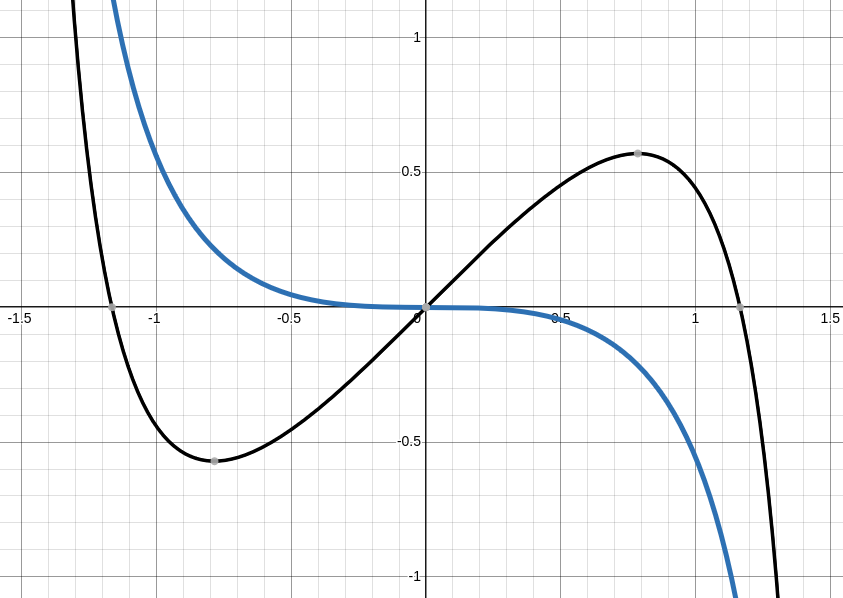
g(x)=tan(x)2x g(x)=\tan(x)-2x

Where g(x)=0g(x) = 0

Plotting this function, we see the zero points are around ±1.166\approx\pm1.166.

I can’t think of any algebra to solve g(x)=0g(x) = 0. Instead, we will use Newton’s method to find some ‘radius of stability’ SS such that g(S)=0g(S)=0

(there’s some humor in here somewhere; I just know it!)

g(x)=tan(x)2xg(x)=sec(x)tan(x)2 \begin{aligned} g(x) &= \tan(x) - 2x\\ g'(x) &= \sec(x)\tan(x) - 2 \end{aligned} vn+1=vntan(vn)2xsec(vn)tan(vn)2 v_{n+1} = v_n - \frac{\tan(v_n)-2x}{\sec(v_n)\tan(v_n)-2}

Starting with g0=1.16g_0 = 1.16, we see it level out to S1.16556118S\approx1.16556118. I do not believe this constant has any simpler symbolic forms.

View Code
from sympy import N, tan, sec

expr = 1.16
for i in range(0, 15):
    expr = expr - (tan(expr) - 2 * expr) / (sec(expr) * tan(expr) - 2)
    # evaluate algebra to numeric value each step to prevent
    # algebraic explosion. Use 200 digits to avoid precision loss
    expr = N(expr, 200)
print(N(expr, 15))

So, around 0π0\pi this well-behaved region is described as

x<S |x| < S

And in general is:

xnπ<S |x - n\pi| < S

Where:

nZS1.16556118 \begin{aligned} n &\in \mathbb{Z}\\ S &\approx1.16556118 \end{aligned}

When gng_n is outside the well-behaved region, gn+1g_{n+1} will skip to be nearby an entirely different multiple of pi. That makes me curious: is there some value of g0g_{0} such that all subsequent gng_n values will keep skipping away and never converge?

Well, there’s the solution g0=Sg_{0} = S where the iterations bounce back and forth, but that’s more of a bounce than a skip. In theory, there exists some value gng_n such that gn+1=gn+πg_{n+1}=g_{n}+\pi. A gng_n of this description will never converge.

xtan(x)+π=x x-\tan(x)+\pi = x tan(x)=π \tan(x) = \pi x=arctan(π) x = \arctan(-\pi)

Of course, this same logic applies for the situation where gn+1=gn±qπg_{n+1} = g_{n} \pm q\pi where qZq\in\mathbb{Z} and q0q\ne 0. So, generally:

arctan(±qπ) \arctan(\pm q\pi)

will diverge. For example:

g0=arctan(2π)g1=arctan(2π)2π \begin{aligned} g_0 &= \arctan(2\pi)\\ g_1 &= \arctan(2\pi)-2\pi \end{aligned}

I was quite interested in describing the nature of this non-well-behaved region. However, the more I looked, the more detail I saw. Slight changes in input create vast differences in output, nudging the inputs even slightly creates entirely different outputs. This detail seems to persist no matter how precise the inputs are.

This all stinks of a fractal.

After discovering that the details were infinite, I stopped trying to directly define the results of the function. However, one last detail I noticed which I have not yet explained is the converging values around π/2-\pi/2 (and all other midpoints between adjacent well-behaved areas)

As seen in the graph, the convergent values around π/2-\pi/2 generally tend to be the multiple of π less than a certain hyperbola. Fascinating.

I recommend viewing this graph in Desmos yourself. I’ve included the code to recreate it below (make sure to make the range on the y-axis quite large).

View Desmos Code

Each line represents a distinct Desmos expression. Copy and paste them into Desmos to import it.

f\left(x\right)=x-\tan\left(x\right)

x=-\frac{\pi}{2}

y=f\left(f\left(f\left(f\left(f\left(f\left(f\left(f\left(f\left(f\left(f\left(f\left(f\left(f\left(f\left(x\right)\right)\right)\right)\right)\right)\right)\right)\right)\right)\right)\right)\right)\right)\right)

\frac{1}{\left(x+\frac{\pi}{2}\right)}

\operatorname{floor}\left(\frac{\frac{1}{\left(x+\frac{\pi}{2}\right)}}{\pi}\right)\pi

In the view, set the x-axis range to

π/20.1xπ/2+0.1 -\pi/2 - 0.1 \leq x \leq -\pi/2 +0.1

and the y-axis range to

100y100 -100 \leq y \leq 100

Perhaps this is quite similar to 3Blue1Brown: Newton’s Fractal. It has been a while since I have seen that video.

Proof that π is rational (joke)

Single Page
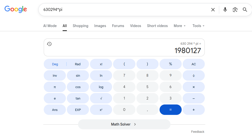
318π999.0366317π208341.0000081630294π1980127.0000017995207π3126535.0000011 \begin{aligned} 318\pi &\approx 999.03\\ 66317\pi &\approx 208341.0000081\\ 630294\pi &\approx 1980127.0000017\\ 995207\pi&\approx 3126535.0000011 \end{aligned}
View Code
from sympy import N, pi, floor
best = (10000, 1)

for i in range(1, 1_000_000):
    val = N(pi * i, 100)
    lz = val - floor(val)
    print(i, lz, val)
    lz = lz.evalf()
    if lz < best[0]:
        best = (lz, i)

print(best)

If I were to trust google’s calculator… then I’d say π is rational.

On A Spigot Algorithm for the Digits of π (Rabinowitz and Wagon)

Single Page

Two equivalent expressions of a standard decimal number:

1.234==1+210+3100+41000=1+110(2+110(3+110(4))) \begin{aligned} 1.234 &=\\ &= 1 + \frac{2}{10} + \frac{3}{100} + \frac{4}{1000}\\ &= 1 + \frac{1}{10}\Big(2 + \frac{1}{10}\Big(3 + \frac{1}{10}\Big(4\Big)\Big)\Big) \end{aligned}

A mixed-radix number is somewhat like having a different base for each digit. The primary objective of this paper is stating mixed-radix representation’s of ee and π\pi, and converting them to more useful bases.

Example of mixed-radix number:

a0+12(a1+13(a2+14(a3+))) a_0 + \frac{1}{2}\Big(a_1 + \frac{1}{3}\Big(a_2 + \frac{1}{4}\Big(a_3 + \ldots\Big)\Big)\Big)

Which expands to

a0+12a1+132a2+1432a3+ a_0 + \frac{1}{2}a_1 + \frac{1}{3 \cdot 2}a_2+ \frac{1}{4\cdot 3\cdot 2}a_3 + \ldots

When ai=1a_i=1 for all ii, this is the well-known power series for ee.

Euler’s number spigot

A. H. J. Sale doi 10.1093/comjnl/11.2.229.

Well-known ee power series:

e=n=01n! e = \sum_{n=0}^{\infty} \frac{1}{n!}

Given in mixed-radix form:

e=1+1(1+12(1+13(1+14(1+(1+1n))))) e = 1 + 1\Big(1 + \frac{1}{2}\Big(1+\frac{1}{3}\Big(1+\frac{1}{4}\Big(1+\ldots\Big(1+\frac{1}{n}\Big)\ldots\Big)\Big)\Big)\Big)

Also can be stated as a recursion:

rn=1+1n(rn+1) r_n = 1+ \frac{1}{n}(r_{n+1})

The paper then multiplies the fractional part of the expression by 1010\frac{10}{10}, and distributes the numerator into the recursion:

e=2+110[12(10+13(10+14(10+15(10+16(10+10())))))] e = 2 + \frac{1}{10} \left[ \frac{1}{2} \Big(10 + \frac{1}{3}\Big(10 + \frac{1}{4}\Big(10 + \frac{1}{5}\Big(10 + \frac{1}{6}\Big(10 + 10(\ldots)\Big)\Big)\Big)\Big)\Big) \right]

The goal of this manipulation is to extract base-10 digits from this mixed-radix form, one digit at a time. We first take this recursion to some specific depth. 55 in this example.

From right to left, we consecutively reduce the inner values mod the outer divisor, moving out the quotient in the process. An example is more clear:

16(10+)=106+6distribute=1+46+6divide and take remainder=1+16(4+)factor \begin{array}{llr} &\frac{1}{6}\left(10+\ldots\right)\\ &= \frac{10}{6} + \frac{\ldots}{6} &\text{distribute}\\ &= 1 + \frac{4}{6} + \frac{\ldots}{6} &\text{divide and take remainder}\\ &= 1 + \frac{1}{6}(4+\ldots) &\text{factor} \end{array}

This method of distributing the divisor, diving with remainder, and factoring is repeated:

e=2+110[7+12(0+13(1+14(0+15(1+16(4+10())))))] e=2+\frac{1}{10}\left[7+\frac{1}{2}\Big(0+\frac{1}{3}\Big(1+\frac{1}{4}\Big(0+\frac{1}{5}\Big(1+\frac{1}{6}\Big(4+10(\ldots)\Big)\Big)\Big)\Big)\Big)\right]

This shows clearly that the 2nd digit is 77. To get further digits, we again multiply the mixed-radix part by 10/1010/10.

e=2+710+1100[12(0+13(10+14(0+15(10+16(40+102())))))] e=2+\frac{7}{10}+ \frac{1}{100}\left[\frac{1}{2}\Big(0+\frac{1}{3}\Big(10+\frac{1}{4}\Big(0+\frac{1}{5}\Big(10+\frac{1}{6}\Big(40+10^2(\ldots)\Big)\Big)\Big)\Big)\Big)\right]

And repeat the process:

e=2+710+1100+1100[12(1+13(1+14(3+15(1+16(4+102())))))] \begin{aligned} e&=2+\frac{7}{10} + \frac{1}{100} \\ &+ \frac{1}{100}\left[\frac{1}{2}\Big(1+\frac{1}{3}\Big(1+\frac{1}{4}\Big(3+\frac{1}{5}\Big(1+\frac{1}{6}\Big(4+10^2(\ldots)\Big)\Big)\Big)\Big)\Big)\right] \end{aligned}

And again:

e=2+710+1102+8103+1103[12(0+13(0+14(1+15(1+16(4+103())))))] \begin{aligned} e&=2+\frac{7}{10} + \frac{1}{10^2} +\frac{8}{10^3}\\ &+ \frac{1}{10^3}\left[\frac{1}{2}\Big(0+\frac{1}{3}\Big(0+\frac{1}{4}\Big(1+\frac{1}{5}\Big(1+\frac{1}{6}\Big(4+10^3(\ldots)\Big)\Big)\Big)\Big)\Big)\right] \end{aligned}

And again:

e=2+710+1102+8103+0104+1104[12(0+13(0+14(1+15(1+16(4+104())))))] \begin{aligned} e&=2+\frac{7}{10} + \frac{1}{10^2}+ \frac{8}{10^3} + \frac{0}{10^4} \\ &+ \frac{1}{10^4}\left[\frac{1}{2}\Big(0+\frac{1}{3}\Big(0+\frac{1}{4}\Big(1+\frac{1}{5}\Big(1+\frac{1}{6}\Big(4+10^4(\ldots)\Big)\Big)\Big)\Big)\Big)\right] \end{aligned}

Which now produces an incorrect result.

e=2.7182e2.7180 \begin{aligned} e &= 2.7182\ldots\\ e &\ne 2.7180\ldots \end{aligned}

Why? Well, it is reasonable to assume that, because we limited the recursion to a finite number of levels, the remaining levels begin to become significant as the powers of 1010 rise.

Looking at the last reasonable result, we see at the end:

4+103() 4 + 10^3(\ldots)

Let’s call ()(\ldots) to be rr , we see

r=17(1+18()) r = \frac{1}{7}\Big(1 + \frac{1}{8}(\ldots)\Big)

Which expands to

r=17!+18!+ r = \frac{1}{7!} + \frac{1}{8!} + \ldots

Multiplying in the 10310^3 creates a value less than 11, and so it does not effect the calculations.

103r=103(17!+18!+)0.227 10^3r = 10^3\left(\frac{1}{7!} + \frac{1}{8!} + \ldots\right) \approx 0.227

However, when the power of ten is increased to 10410^4, we see:

104(17!+18!+)2.267 10^4\left(\frac{1}{7!} + \frac{1}{8!} + \ldots\right) \approx 2.267

Which is greater than one and will likely cause a deleterious effect when it is missing from the calculations. So, the question is: how many terms does the recursion need to be expanded to to obtain dd digits? Instead of thinking about the algorithm as algebraic manipulations on a recursive equation, I find it easier to think of as an array of numbers. The first step of the above example becomes:

i01234n23456v1010101010q74321r01014 \begin{array}{c:rrrrr} i & \small0 & \small1 & \small2 & \small3 & \small4 \\ n &\small 2 &\small 3 &\small 4 &\small 5 &\small 6 \\ \hline v &10 & 10 & 10 & 10 & 10 \\ q & 7 & 4 & 3 & 2 & 1 \\ r & 0 & 1 & 0 & 1 & 4 \\ \end{array}

Where:

iindexni=i+2divisorvivalueqi=(vi+qi+1)/niquotientri=(vi+qi+1)modniremainderq0=output digit \begin{array}{llll} i & & \text{index}\\ n_i &= i+2 & \text{divisor}\\ v_i & & \text{value}\\ q_i &= \lfloor (v_i+q_{i+1})/n_i \rfloor & \text{quotient}\\ r_i &= (v_i+q_{i+1}) \mod n_i &\text{remainder}\\ \hline\\ q_0 &= \text{output digit} \end{array}

Inside the array, there are 5 slots (columns). Each slot represents a level of recursion. More slots => more digits extractable.

Let dd represent the number of digits being extracted, and ss represent the number of slots. A calculation using ss slots will yield dd digits when the following is true:

1>10d(x=s+21x!) 1 > 10^d\left(\sum_{x=s+2}^{\infty} \frac{1}{x!} \right)

Infinite sums are cumbersome so instead a simpler form is desired. So long as the value of the sum overestimated, a simpler form will still work.

The following form is valid according to Desmos and WolframAlpha, so I’ll trust those sites on that.

1(s+1)!>x=s+21x! \frac{1}{(s+1)!} \gt \sum_{x=s+2}^{\infty} \frac{1}{x!}

Substituting this simpler expression in:

(s+1)!>10d (s+1)! > 10^d

Solve for digits:

ln((s+1)!)ln(10)>d \frac{\ln((s+1)!)}{\ln(10)} > d

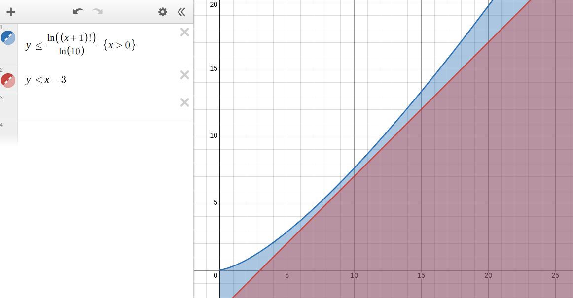
Plotting this, we see

The linear approximation of

ds3 d \le s-3

Fits well under the entire domain. This approximation becomes poorer as more slots are added, but never overestimates. When s=70s=70, d100d \le \approx100

A polynomial or piecewise approximation could provide improvement. The original paper provides a different approximation entirely. I have not reviewed that approximation.

When in one of the previous examples the result of 2.71802.7180\ldots was obtained, only 5 slots were used, and so only two digits after the decimal place should have been expected with confidence to be correct.


Back again to thinking of the problem algorithmically:

i01234n23456v1010101010q74321r01014 \begin{array}{c:rrrrr} i & \small0 & \small1 & \small2 & \small3 & \small4 \\ n &\small 2 &\small 3 &\small 4 &\small 5 &\small 6 \\ \hline v &10 & 10 & 10 & 10 & 10 \\ q & 7 & 4 & 3 & 2 & 1 \\ r & 0 & 1 & 0 & 1 & 4 \\ \end{array}

Where:

iindexni=i+2divisorvivalueqi=(vi+qi+1)/niquotientri=(vi+qi+1)modniremainderq0=nth digit of e \begin{array}{llll} i & & \text{index}\\ n_i &= i+2 & \text{divisor}\\ v_i & & \text{value}\\ q_i &= \lfloor (v_i+q_{i+1})/n_i \rfloor & \text{quotient}\\ r_i &= (v_i+q_{i+1}) \mod n_i &\text{remainder}\\ \hline\\ q_0 &= n^{\text{th}} \text{ digit of } e\\ \end{array}

To find the second digit, update the table such that:

Then apply the same rules, stopping after i=1i=1:

i01234n23456v01001040q13036r01314 \begin{array}{c:rrrrr} i & \small0 & \small1 & \small2 & \small3 & \small4 \\ n &\small 2 &\small 3 &\small 4 &\small 5 &\small 6 \\ \hline v & 0 & 10 & 0 & 10 & 40 \\ q & 1 & 3 & 0 & 3 & 6 \\ r & 0 & 1 & 3 & 1 & 4 \\ \end{array}

And so digit #2 is 11: 2.712.71\ldots.

An implementation in Rust is provided.

View Implementation
fn main() {
    for i in 1..20 {
        println!("{:?}", e(i));
    }
}

fn e(d: u32) -> Vec<u8> {
    let mut digits = vec![0; d as usize];
    let slots = d as usize + 3;
    let mut tmp = vec![10; slots];
    for stop in 0..d as usize {
        let mut carry = 0;
        for i in (0..slots).rev() {
            let n = i as u32 + 2;
            let s = carry + tmp[i];
            let q = s / n;
            let r = s % n;
            tmp[i] = r * 10;
            carry = q;
        }
        digits[stop] = carry as u8;
    }
    digits
}

This implementation seems very similar to the Algol 60 one provided in the paper. I’m not familiar with the array syntax and semantics in Algol 60, so there may be variation there.

Back to π

After a slight detour, the study of π is resumed.

Todo….

Geometric Integer Sums of Lines and Squares

Single Page

On the sums of natural numbers

Let Ln=1+2+3++n=? \text{Let } L_n = 1 + 2 + 3 + \ldots + n = ?

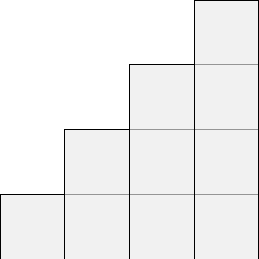
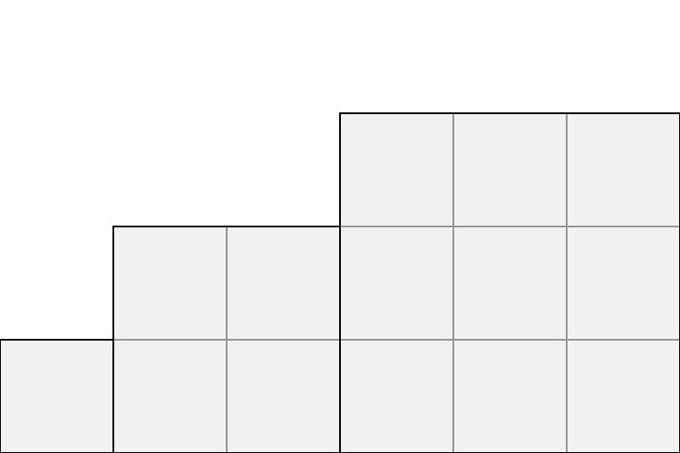
Think about each integer as an area, and draw each component integer of LnL_n ascending, in a square of dimension nn:

In this case, n=4n=4 and L4=10L_4 = 10.

Notice the diagonal set of squares from the bottom left to the top right of the greater square. There exist nn units on this diagonal. Above the diagonal, there are zero units as part of the greater square. Below the diagonal, all units are part of the greater square.

We know the diagonal has a total area of nn, but what about the area under the diagonal? If we consider the greater square with the diagonal removed, then this under-area is clearly half of the greater square’s (sans diagonal) area.

Thus the area of the under-area is n2n2\frac{n^2 -n}{2} units

To find L4L_4, the diagonal must be added back

L4=n2n2+n=n2+n2 L_4 = \frac{n^2 - n}{2} + n = \frac{n^2 + n}{2}

Proof By Induction

Base condition:

L1=1+12=1 L_1 = \frac{1+1}{2} = 1

Following values

Ln+1=Ln+n+1 L_{n+1} = L_{n} + n + 1 (n+1)2+n2=n2+n2+n+1 \frac{(n+1)^2 + n}{2} = \frac{n^2+n}{2} + n + 1

Expand left side

n2+2n+1+n+12=n2+n2+n+1 \frac{n^2+2n+1 + n + 1}{2} = \frac{n^2+n}{2} + n + 1

Both sides are equal.

On the sums of squares of natural numbers

Let Sn=1+22+32++n2=? \text{Let } S_n = 1 + 2^2 + 3^2 + \ldots + n^2 = ?

Or recursively:

Sn=Sn1+n2 S_n = S_{n-1} + n^2

(Note, this section follows from a YouTube video by Perfect Yarn)

Thing about each squared integer as a square. Arrange them ascending:

In this case, n=3n = 3 and S3=14S_3 = 14.

Just as with the un-squared natural numbers, a closed form for SnS_n can be found by interpreting this geometric construction.

If a equation for the quantity of units in each row RjR_{j} is found, then the total SnS_n is the sum of the row RjR_{j} values. Where jj is the row number, from bottom up, starting at 00:

Sn=R0+R1++Rn1 S_n = R_{0} + R_{1} + \ldots + R_{n-1}

For the bottom row ( j=0j=0), R0,3=L3R_{0,3} = L_3 (where LnL_n is the sum of natural numbers from 1…n) or

R0,3=32+32 R_{0,3} = \frac{3^2+3}{2}

For the following values of j>0j > 0, RjR_{j} will decrease. Each increase of jj will cause a subsequent quantity to be removed:

Rj=n2+n2j2+j2 R_{j} = \frac{n^2+n}{2} - \frac{j^2+j}{2}

Again, recall that

Sn=R0+R1++Rn1 S_n = R_{0} + R_{1} + \ldots + R_{n-1}

Substituting in, RjR_{j} we see:

Sn=n(n2+n2)02+0212+12(n1)2+(n1)2 S_n = n\left(\frac{n^2+n}{2}\right) - \frac{0^2+0}{2} - \frac{1^2+1}{2} - \ldots - \frac{(n-1)^2+(n-1)}{2}

Factor

Sn=12(n(n2+n)(02+12++(n1)2)(0+1++(n1))) S_n = \frac{1}{2}\left(n\left({n^2+n}\right) - (0^2 + 1^2 + \ldots + (n-1)^2) - (0 + 1 + \ldots + (n-1))\right)

The sum of natural numbers of the right of the equation can be simplified to Ln1L_{n-1} and the sum of squares on the left can be simplified to Sn1S_{n-1}

Sn=12(n(n2+n)Sn1(n1)2+(n1)2) S_n = \frac{1}{2}\left(n\left({n^2+n}\right) - S_{n-1} - \frac{(n-1)^2+(n-1)}{2}\right)

Recall that:

Sn=Sn1+n2Sn1=n2Sn \begin{aligned} S_n &= S_{n-1} + n^2\\ S_{n-1} &= n^2 - S_n\\ \end{aligned}

Substitute Sn1S_{n-1}

Sn=12(n(n2+n)Sn+n2(n1)2+(n1)2) S_n = \frac{1}{2}\left(n\left({n^2+n}\right) - S_n + n^2 - \frac{(n-1)^2+(n-1)}{2}\right)

Factor SnS_n to one side

Sn=13(n(n2+n)+n2(n1)2+(n1)2) S_n = \frac{1}{3}\left(n\left({n^2+n}\right) + n^2 - \frac{(n-1)^2+(n-1)}{2}\right)

Simplify

Sn=13n(n2+32n+12) S_n = \frac{1}{3}n\left(n^2+\frac{3}{2}n + \frac{1}{2}\right)

Sn=16n(2n2+3n+1) S_n = \frac{1}{6}n\left(2n^2+3n + 1\right)

Proof By Induction

Base condition

S1=16(212+31+1)=66=1 S_1 = \frac{1}{6}\left(2\cdot 1^2 +3\cdot 1 + 1\right) = \frac{6}{6} = 1

Following values

Sn+1=Sn+(n+1)2 S_{n+1} = S_n + (n+1)^2 16(n+1)(2(n+1)2+3(n+1)+1)=16n(2n2+3n+1)+(n+1)2 \frac{1}{6}(n+1)\left(2(n+1)^2+3(n+1) + 1\right) = \frac{1}{6}n\left(2n^2+3n + 1\right) + (n+1)^2

Simplify

(n+1)(2n2+7n+6)=n(2n2+3n+1)+6n2+12n+6 (n+1)\left(2n^2+7n+6\right) = n\left(2n^2+3n + 1\right) + 6n^2+12n+6

2n3+9n2+13n+6=2n3+9n2+13n+6 2n^3+9n^2+13n+6 = 2n^3+9n^2 +13n+ 6

Both sides are equal.

Polynomial Integer Sums as Functional Equations

Single Page

The sum of natural numbers

Ln=1+2+3++n L_n = 1 + 2 + 3 + \ldots + n

Can be described as a recursive function

f(x)=x+f(x1) f(x) = x + f(x-1)

Or

f(x)f(x1)=x f(x) - f(x-1) = x

We seek f(x)f(x). We will start with a guess-and-check method starting with f(x)=x2f(x) = x^2.

Guess:f(x)=x2x2(x1)2=?xx2x2+2x1x \begin{array}{rlcc} \text{Guess:} & f(x) = x^2\\ \Rightarrow& x^2 - (x-1)^2 &\stackrel{?}{=} &x\\ \Rightarrow& \cancel{x^2} - \cancel{x^2} + 2x - 1 &\ne &x \end{array}

This guess for f(x)f(x) does not satisfy the constraint and must be updated. A more clear method for doing this will be explained later, for now, halve current guess:

Guess:f(x)=12x212x212(x1)2=?x12x212x2+x12x \begin{array}{rlcc} \text{Guess:} & f(x) = \frac{1}{2}x^2\\ \Rightarrow& \frac{1}{2}x^2 - \frac{1}{2}(x-1)^2 &\stackrel{?}{=} &x\\ \Rightarrow& \cancel{\frac{1}{2}x^2} - \cancel{\frac{1}{2}x^2} + x - \frac{1}{2} &\ne &x \end{array}

Now, the guess for f(x)f(x) is a lot closer to satisfying the equation. Update guess again

Guess:f(x)=12x2+12x12x2+12x12(x1)212(x1)=?x12x2+12x12x2+x+12x12+12=x \begin{array}{rlcc} \text{Guess:} & f(x) = \frac{1}{2}x^2 + \frac{1}{2}x\\ \Rightarrow& \frac{1}{2}x^2 + \frac{1}{2}x - \frac{1}{2}(x-1)^2 - \frac{1}{2}(x-1) &\stackrel{?}{=} &x\\ \Rightarrow& \cancel{\frac{1}{2}x^2} + \cancel{\frac{1}{2}x} - \cancel{\frac{1}{2}x^2} +x + \cancel{\frac{1}{2}x} - \cancel{\frac{1}{2}} + \cancel{\frac{1}{2}} &= &x \end{array}

A Bit more formally

This method, as previously shown, works by incrementally adding and removing polynomials to f(x)f(x) until

f(x)f(x1)=h(x) f(x) - f(x-1) = h(x)

Where h(x)h(x) is some polynomial function. A table has been made to better understand the effect which adding a power of xx to the guess for f(x)f(x) has on the overall equation.

x1x22x1x33x33x+1 \begin{array}{lll} x & \Rightarrow &1 \\ x^2 & \Rightarrow &2x -1\\ x^3 & \Rightarrow &3x^3 -3x+1\\ \end{array}

The above table indicates that, if x2x^2 is added to the guess for f(x)f(x), then f(x)f(x1)f(x)-f(x-1) will have 2x12x-1 added to it as a result.

Using this table, the method will again be applied to the sum of squares, where h(x)=x2h(x) = x^2. It is not necessary to use the table, but the algebra becomes pretty murky without it.

The starting guess for f(x)f(x) is informed by the highest power of xx in h(x)h(x). Because h(x)=x2h(x)=x^2, the first guess will be f(x)=13x3f(x) = \frac{1}{3}x^3. The specific 13x3\frac{1}{3}x^3 is chosen because it will make f(x)f(x1)f(x) - f(x-1) contain x2x^2 which is of course desirable.

Guess:f(x)=13x313x313(x1)3=?x2x2x+13x2 \begin{array}{rlcc} \text{Guess:} & f(x) = \frac{1}{3}x^3\\ \Rightarrow& \frac{1}{3}x^3 - \frac{1}{3}(x-1)^3 &\stackrel{?}{=} &x^2\\ \Rightarrow& x^2 - x + \frac{1}{3} &\ne &x^2 \end{array}

Now that the expression contains x2x^2, the unnecessary components x+13-x + \frac{1}{3} must be removed. Remove x-x by adding 12x2\frac{1}{2}x^2 to the guess for f(x)f(x)

Guess:f(x)=13x3+12x213x3+12x213(x1)313(x1)2=?x2x2x+13+x12x2 \begin{array}{rlcc} \text{Guess:} & f(x) = \frac{1}{3}x^3 + \frac{1}{2}x^2\\ \Rightarrow& \frac{1}{3}x^3 + \frac{1}{2}x^2 - \frac{1}{3}(x-1)^3 - \frac{1}{3}(x-1)^2 &\stackrel{?}{=} &x^2\\ \Rightarrow& x^2 - \cancel{x} + \frac{1}{3} + \cancel{x} - \frac{1}{2} &\ne &x^2 \end{array}

Next, 16-\frac{1}{6} is removed by adding 16x\frac{1}{6}x to the guess for f(x)f(x)

Guess:f(x)=13x3+12x2+16x13x3+12x2+16x13(x1)313(x1)216(x1)=?x2x216+16=x2 \begin{array}{rlcc} \text{Guess:} & f(x) = \frac{1}{3}x^3 + \frac{1}{2}x^2 + \frac{1}{6}x\\ \Rightarrow& \frac{1}{3}x^3 + \frac{1}{2}x^2 + \frac{1}{6}x - \frac{1}{3}(x-1)^3 - \frac{1}{3}(x-1)^2 - \frac{1}{6}(x-1) &\stackrel{?}{=} &x^2\\ \Rightarrow& x^2 - \cancel{\frac{1}{6}} + \cancel{\frac{1}{6}} &= &x^2 \end{array}

Thus, the sum of squares formula is

f(x)=13x3+12x2+16x f(x) = \frac{1}{3}x^3 + \frac{1}{2}x^2 + \frac{1}{6}x

Solver Algorithm Implementation

A sample algorithm implementation in Python using NumPy is provided:

View Code
import fractions as F
from numpy.polynomial import polynomial as P

# Possibly unexpected behavior:
assert P.polytrim([0]) == [0]

def polyset(p, n, v):
    while len(p) <= n:
        p.append(0)
    p[n] = v

# Given f(x) - f(x-1) = g(x) Where `g` is given value
given = [F.Fraction(0), F.Fraction(1)] # x^2

# Populate table
table = []
base = [F.Fraction(-1), F.Fraction(1)]
tmp = base.copy()
for i in range(len(given) + 1):
    x = tmp[:-1]
    x = P.polymul(x, [-1])
    leading_coef = x[-1]
    table.append((leading_coef, x))
    tmp = P.polymul(tmp, base)
tmp = None
base = None

# move given to left side of equation: f(x)-f(x-1) - g(x) = 0
working = P.polymul(given, -1)
out = []

# Work until a satisfying function $f$ is found
# such that the equation is zero on both sides
while len(working) > 1 or working[-1] != 0:
    high_pwr = len(working) - 1
    hp_c = working[high_pwr]
    assert hp_c != 0
    lc, tp = table[high_pwr]
    factor = hp_c / lc * -1
    polyset(out, high_pwr + 1, factor)
    tp = P.polymul(tp, [factor])
    working = P.polyadd(working, tp)
    working = P.polytrim(working)

print("The sum of: ", P.Polynomial(given))
print("Has the closed form: ", P.Polynomial(out))

Additionally, I’ve ported it to JavaScript so you can use it interactively. All polynomials must be ine expanded form.

Interactive Solver
(e.g: x^2 + 2/3x^3 - 3)
Parsed as:
Output: