Newton’s Method Pi

Suppose $f(x)=\sin(x)$, then $f(\pi) = 0$. Using Newton’s method, we arrive at the recursion:

Which gives π accurate to 100 digits in only 5 iterations.

from sympy import N, tan, pi

expr = 3
for i in range(0, 5):
    expr = expr - tan(expr)

print(N(expr, 100))
print(N(pi - expr, 100))

The behavior of $g_{n+1} = g_n - \tan(g_n)$ depends highly the initial value $g_0$. This makes some intuitive sense because $\sin(x)$ has many different roots so the sequence would likely converge to the nearest root to the starting point.

This behavior is clear by plotting $f(x) = x - \tan(x)$:

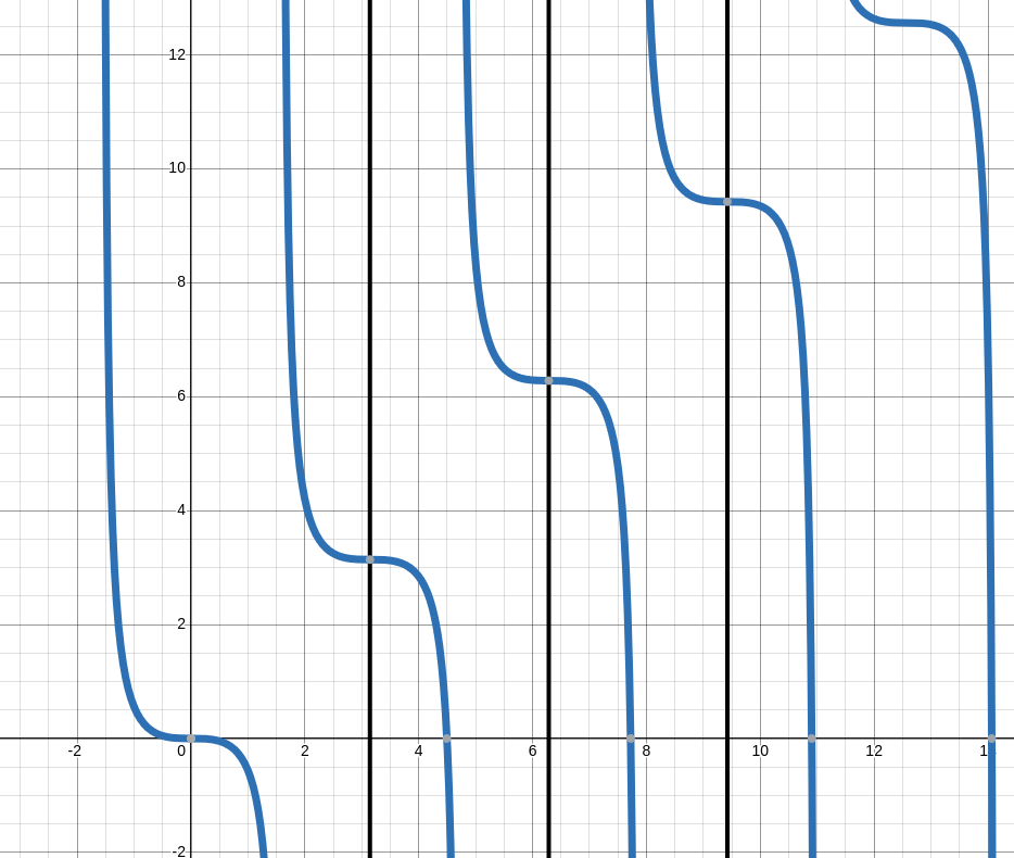
Around each multiple of pi, the graph flattens out. to the right of each flat point, the value of the function is decreases slightly. To the left, the value increases slightly. When the function is interpreted as the mapping from the previous value $x$ to the next value $f(x)$, the slight decreases and increases near each multiple of π makes the recursion stably approach the nearest multiple of π. Further away from the multiples of π, the slope becomes steep enough to ‘push’ the next step of the recursion away from the nearest multiple of pi. The steep region is not well-behaved. for these notes, ‘well-behaved’ means that the recursion $g_{n+1} = g_n - \tan(g_n)$ has a value which approaches the multiple of π nearest to $g_0$.

Specifically, let’s look at $x=0\pi$. The well-behaved region will extend an equal distance positive and negative from zero (because the function is symmetric to an extent around the multiples of π) Therefore, we can solve for this distance by finding $g_n = g_{n+1}$, or $x=-(x-tan(x))$.

Or

Where $g(x) = 0$

Plotting this function, we see the zero points are around $\approx\pm1.166$.

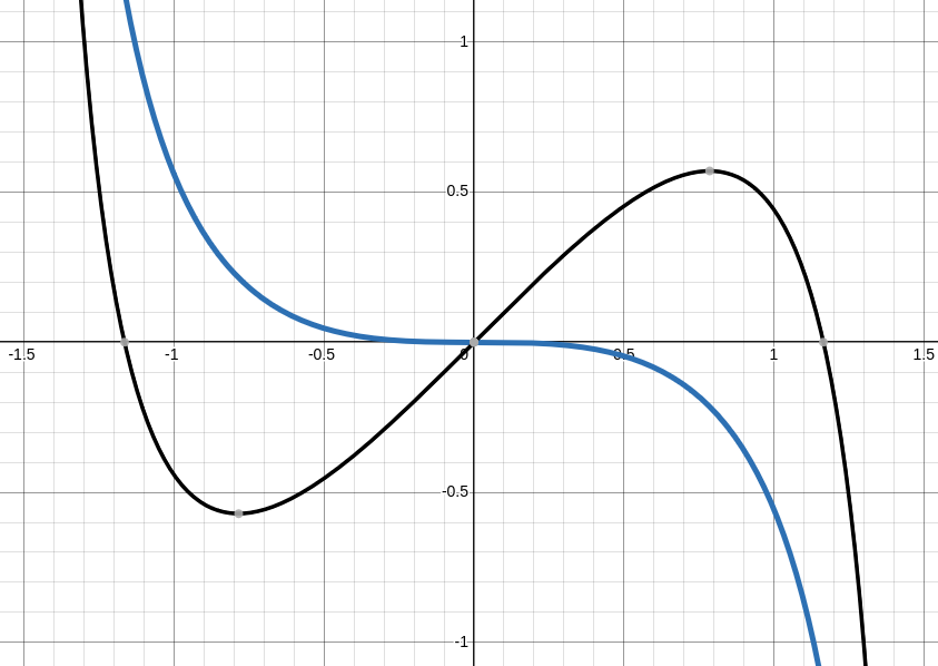
I can’t think of any algebra to solve $g(x) = 0$. Instead, we will use Newton’s method to find some ‘radius of stability’ $S$ such that $g(S)=0$

(there’s some humor in here somewhere; I just know it!)

Starting with $g_0 = 1.16$, we see it level out to $S\approx1.16556118$. I do not believe this constant has any simpler symbolic forms.

from sympy import N, tan, sec

expr = 1.16
for i in range(0, 15):
    expr = expr - (tan(expr) - 2 * expr) / (sec(expr) * tan(expr) - 2)
    # evaluate algebra to numeric value each step to prevent
    # algebraic explosion. Use 200 digits to avoid precision loss
    expr = N(expr, 200)
print(N(expr, 15))

So, around $0\pi$ this well-behaved region is described as

And in general is:

Where:

When $g_n$ is outside the well-behaved region, $g_{n+1}$ will skip to be nearby an entirely different multiple of pi. That makes me curious: is there some value of $g_{0}$ such that all subsequent $g_n$ values will keep skipping away and never converge?

Well, there’s the solution $g_{0} = S$ where the iterations bounce back and forth, but that’s more of a bounce than a skip. In theory, there exists some value $g_n$ such that $g_{n+1}=g_{n}+\pi$. A $g_n$ of this description will never converge.

Of course, this same logic applies for the situation where $g_{n+1} = g_{n} \pm q\pi$ where $q\in\mathbb{Z}$ and $q\ne 0$. So, generally:

will diverge. For example:

I was quite interested in describing the nature of this non-well-behaved region. However, the more I looked, the more detail I saw. Slight changes in input create vast differences in output, nudging the inputs even slightly creates entirely different outputs. This detail seems to persist no matter how precise the inputs are.

This all stinks of a fractal.

After discovering that the details were infinite, I stopped trying to directly define the results of the function. However, one last detail I noticed which I have not yet explained is the converging values around $-\pi/2$ (and all other midpoints between adjacent well-behaved areas)

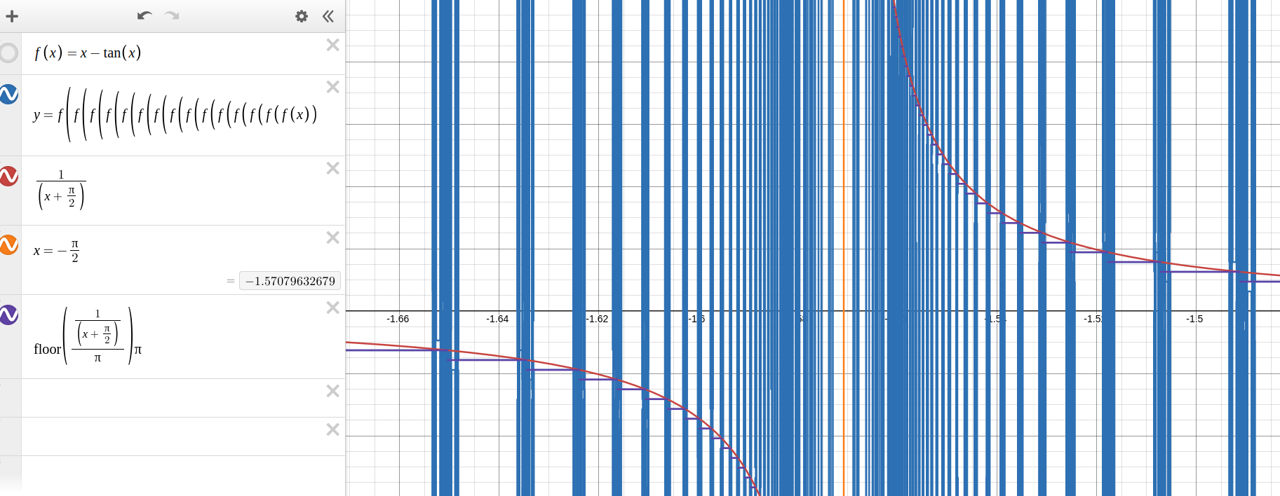
As seen in the graph, the convergent values around $-\pi/2$ generally tend to be the multiple of π less than a certain hyperbola. Fascinating.

I recommend viewing this graph in Desmos yourself. I’ve included the code to recreate it below (make sure to make the range on the y-axis quite large).

f\left(x\right)=x-\tan\left(x\right)

x=-\frac{\pi}{2}

y=f\left(f\left(f\left(f\left(f\left(f\left(f\left(f\left(f\left(f\left(f\left(f\left(f\left(f\left(f\left(x\right)\right)\right)\right)\right)\right)\right)\right)\right)\right)\right)\right)\right)\right)\right)

\frac{1}{\left(x+\frac{\pi}{2}\right)}

\operatorname{floor}\left(\frac{\frac{1}{\left(x+\frac{\pi}{2}\right)}}{\pi}\right)\pi

Perhaps this is quite similar to 3Blue1Brown: Newton’s Fractal. It has been a while since I have seen that video.