This note is one of many taken during 2026

On Newton’s Method

May 22nd 2026

Newton’s method allows finding the ‘root’ of a function (where it is zero), given conditions expressed in the wikipedia article no doubt.

More than this however, it can be used to find the inverse of a function. The common example is $\sqrt{2}$ . If you know $x$ where $x^2-2=0$ , then you know $\sqrt{2}$ .

The rough gist of the algorithm is as follows.

Take a function like $f(x) = x^2-2$
Make an arbitrary guess on the value of $x$ where $f(x)=0$ , $g_0$
Evaluate $f(x)$ at $g_0$ and find the line tangent to $f(x)$ at $g_0$
Find the x-intercept of the tangent line. This x-intercept value is $g_1$
Repeat steps 2…5 (incrementing $n$ throughout) until a satisfactory precision is obtained.

Algebraically, we start with the function and its derivative:

\begin{aligned} f(x)&=x^2-2 & f'(x)&=2x \end{aligned}

And make a guess $g_0$ and create the tangent line at that guess location on $f(x)$

y = f'(g_0)x + b

find $b$ by evaluating at $g_0$ :

f'(g_0)g_0 + b = f(g_0)

b = f(g_0) - f'(g_0)g_0

Which finishes the line equation as:

y = f'(g_0)x + f(g_0) - f'(g_0)g_0

Next, find the x-coordinate by evaluating at $y=0$

\begin{aligned} 0 &= f'(g_0)x + f(g_0) - f'(g_0)g_0\\ f'(g_0)g_0-f(g_0) &= f'(g_0)x\\ g_0 - \frac{f(g_0)}{f'(g_0)} &= x \end{aligned}

As stated above, this $x$ value is actually $g_1$ , or generally

g_{n+1} = g_n - \frac{f(g_n)}{f'(g_n)}

Going back the case of $\sqrt{2}$ , we substitute in the function

g_{n+1} = g_n - \frac{{g_n}^2-2}{2g_n}

With $g_n=5$ we see the first four approximations as:

\begin{array}{ccc} g_0 &= &5\\ g_1 &= &2.7\\ g_2 &\approx &1.7204\\ g_3 &\approx &1.4415\\ g_4 &\approx &1.4145\\ \end{array}

Generally…

This process is easily generalized to finding inverses instead of roots — just as in the $\sqrt{2}$ example.

$f(x)$ was previously defined as $x^2-2$ , but more generically is described as $f(x)=x^2$ . Then, inside the recursive equation, the $-2$ is placed outside the function

g_{n+1} = g_n - \frac{f(g_n) - 2}{f'(g_n)}

The above $g_{n+1}$ approximates $f^{-1}(2)$ . the $2$ is replaced with some constant $c$ to find $f^{-1}(c)$ :

The generic case for $\sqrt{c}$ then is:

g_{n+1} = g_{n} - \frac{{g_n}^2 -c}{2g_n}

\begin{aligned} g_{n+1} &= g_n - \frac{{g_n}^2-c}{2g_n}\\ \lim_{n \to \infty} {g_{n}} &= \sqrt{c} \end{aligned}

One way to loosely verify this is to: consider that when $n$ approaches $\infty$ , the differences between $g_n$ and $g_{n+1}$ will grow increasingly smaller (assuming the limit does indeed converge) and indeed will be come so close that we can consider them to be equal. So, we set $g_{n+1} = g_n = x$ and solve:

\begin{aligned} x &= x - \frac{x^2-c}{2x}\\ \frac{x^2-c}{2x} &= 0 \\ x^2 &= c\\ x &= \sqrt{c} \end{aligned}

Other inverses

This method can be extended to other functions. Some examples:

\begin{array}{rcl} \ln(x) & \Rightarrow & g_{n+1} = g_n - 1 + \frac{x}{e^{g_n}} \\ \log_2(x) & \Rightarrow & g_{n+1} = g_n - 1 + \frac{x}{2^{g_n}\ln(2)} \\ x & \Rightarrow & g_{n+1} = g_n - g_n + x \end{array}

Approximate Functions

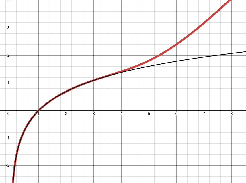
By expanding the recursion a few steps, we can create an obnoxious approximation for $\ln(x)$ :

\ln(x) \approx x e^{1 - x} + x e^{- x e^{1 - x} - x + 2} + x e^{- x e^{1 - x} - x e^{- x e^{1 - x} - x + 2} - x + 3} + x - 4

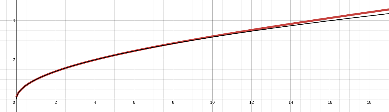
And one for $\sqrt{x}$ :

\sqrt{x}\approx\frac{0.0625 x^{4} + 1.75 x^{3} + 4.375 x^{2} + 1.75 x + 0.0625}{0.5 x^{3} + 3.5 x^{2} + 3.5 x + 0.5}

In a way, this approximation for $\sqrt{x}$ is quite reasonably constructed. It has plenty of detail around the origin, but as it goes further the higher-order polynomial components divide out and all that is left is the slope asymptote.

These examples were generated with the Python library SymPy. (I got exhausted of writing it by hand around third recursion)

View Code

from sympy import symbols, simplify, print_latex

x = symbols("x")

expr = 1
for i in range(0, 3):
    expr = 0.5 * expr + x / (2 * expr)

print_latex(simplify(expr))

This note is one of many taken during 2026