As stated above, this
x value is actually
g1, or generally
gn+1=gn−f′(gn)f(gn)
Going back the case of
2, we substitute in the function
gn+1=gn−2gngn2−2
With
gn=5 we see the first four approximations as:
g0g1g2g3g4==≈≈≈52.71.72041.44151.4145
Generally…
This process is easily generalized to finding inverses instead of roots — just as in the
2 example.
f(x) was previously defined as
x2−2, but more generically is described as
f(x)=x2. Then, inside the recursive equation, the
−2 is placed outside the function
gn+1=gn−f′(gn)f(gn)−2
The above
gn+1 approximates
f−1(2). the
2 is replaced with some constant
c to find
f−1(c):
The generic case for
c then is:
gn+1=gn−2gngn2−c
Or
gn+1n→∞limgn=gn−2gngn2−c=c
One way to loosely verify this is to: consider that when
n approaches
∞, the differences between
gn and
gn+1 will grow increasingly smaller (assuming the limit does indeed converge) and indeed will be come so close that we can consider them to be equal. So, we set
gn+1=gn=x and solve:
x2xx2−cx2x=x−2xx2−c=0=c=c
Other inverses
This method can be extended to other functions. Some examples:
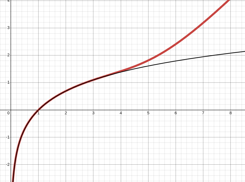
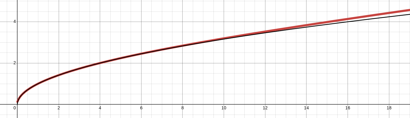
In a way, this approximation for
x is quite reasonably constructed.
It has plenty of detail around the origin, but as it goes further the higher-order polynomial components divide out and all that is left is the slope asymptote.
These examples were generated with the Python library SymPy. (I got exhausted of writing it by hand around third recursion)
The behavior of
gn+1=gn−tan(gn) depends highly the initial value
g0.
This makes some intuitive sense because
sin(x) has many different roots so the sequence would likely converge to the nearest root to the starting point.
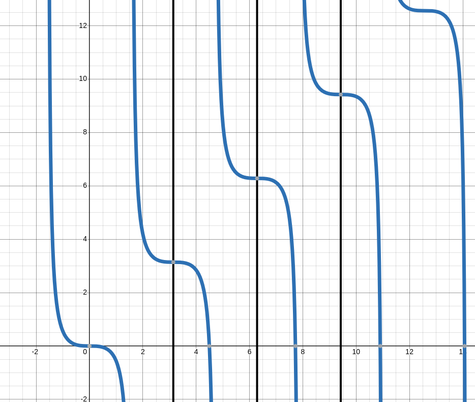
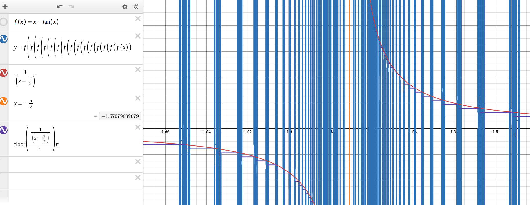
This behavior is clear by plotting
f(x)=x−tan(x):
Around each multiple of pi, the graph flattens out.
to the right of each flat point, the value of the function is decreases slightly.
To the left, the value increases slightly.
When the function is interpreted as the mapping from the previous value
x to the next value
f(x), the slight decreases and increases near each multiple of π makes the recursion stably approach the nearest multiple of π.
Further away from the multiples of π, the slope becomes steep enough to ‘push’ the next step of the recursion away from the nearest multiple of pi. The steep region is not well-behaved.
for these notes, ‘well-behaved’ means that the recursion
gn+1=gn−tan(gn) has a value which approaches the multiple of π nearest to
g0.
Specifically, let’s look at
x=0π.
The well-behaved region will extend an equal distance positive and negative from zero (because the function is symmetric to an extent around the multiples of π)
Therefore, we can solve for this distance by finding
gn=gn+1, or
x=−(x−tan(x)).
2x=tan(x)
Or
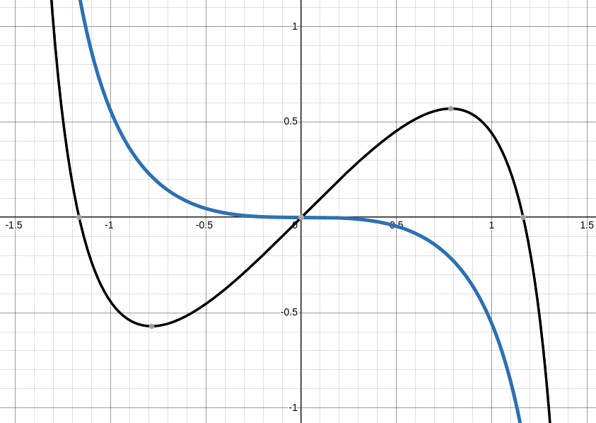
g(x)=tan(x)−2x
Where
g(x)=0
Plotting this function, we see the zero points are around
≈±1.166.
I can’t think of any algebra to solve
g(x)=0.
Instead, we will use Newton’s method to find some ‘radius of stability’
S such that
g(S)=0
(there’s some humor in here somewhere; I just know it!)
Starting with
g0=1.16, we see it level out to
S≈1.16556118.
I do not believe this constant has any simpler symbolic forms.
View Code
fromsympyimportN,tan,secexpr=1.16foriinrange(0,15):expr=expr-(tan(expr)-2*expr)/(sec(expr)*tan(expr)-2)# evaluate algebra to numeric value each step to prevent# algebraic explosion. Use 200 digits to avoid precision lossexpr=N(expr,200)print(N(expr,15))
So, around
0π this well-behaved region is described as
∣x∣<S
And in general is:
∣x−nπ∣<S
Where:
nS∈Z≈1.16556118
When
gn is outside the well-behaved region,
gn+1 will skip to be nearby an entirely different multiple of pi.
That makes me curious: is there some value of
g0 such that all subsequent
gn values will keep skipping away and never converge?
Well, there’s the solution
g0=S where the iterations bounce back and forth, but that’s more of a bounce than a skip.
In theory, there exists some value
gn such that
gn+1=gn+π.
A
gn of this description will never converge.
x−tan(x)+π=xtan(x)=πx=arctan(−π)
Of course, this same logic applies for the situation where
gn+1=gn±qπ where
q∈Z and
q=0.
So, generally:
arctan(±qπ)
will diverge. For example:
g0g1=arctan(2π)=arctan(2π)−2π
I was quite interested in describing the nature of this non-well-behaved region.
However, the more I looked, the more detail I saw.
Slight changes in input create vast differences in output, nudging the inputs even slightly creates entirely different outputs.
This detail seems to persist no matter how precise the inputs are.
This all stinks of a fractal.
After discovering that the details were infinite, I stopped trying to directly define the results of the function.
However, one last detail I noticed which I have not yet explained is the converging values around
−π/2 (and all other midpoints between adjacent well-behaved areas)
As seen in the graph, the convergent values around
−π/2 generally tend to be the multiple of π less than a certain hyperbola. Fascinating.
I recommend viewing this graph in Desmos yourself.
I’ve included the code to recreate it below
(make sure to make the range on the y-axis quite large).
View Desmos Code
Each line represents a distinct Desmos expression.
Copy and paste them into Desmos to import it.
A mixed-radix number is somewhat like having a different base for each digit.
The primary objective of this paper is stating mixed-radix representation’s of
e and
π, and converting them to more useful bases.
Example of mixed-radix number:
a0+21(a1+31(a2+41(a3+…)))
Which expands to
a0+21a1+3⋅21a2+4⋅3⋅21a3+…
When
ai=1 for all
i, this is the well-known power series for
e.
The goal of this manipulation is to extract base-10 digits from this mixed-radix form, one digit at a time.
We first take this recursion to some specific depth.
n=6 in this example.
From right to left, we consecutively reduce the inner values mod the outer divisor, moving out the quotient in the process.
An example is more clear:
61(10+…)=610+6…=1+64+6…=1+61(4+…)distributedivide and take remainderfactor
This method of distributing the divisor,
diving with remainder, and factoring is repeated:
Why? Well, it is reasonable to assume that, because we limited the recursion to a finite number of levels,
the remaining levels begin to become significant as the powers of
10 rise.
Looking at the last reasonable result, we see at the end:
4+103(…)
Let’s call
(…) to be
r , we see
r=71(1+81(…))
Which expands to
r=7!1+8!1+…
Multiplying in the
103 creates a value less than
1, and so it does not effect the calculations.
103r=103(7!1+8!1+…)≈0.227
However, when the power of ten is increased to
104, we see:
104(7!1+8!1+…)≈2.267
Which is greater than one and will likely cause a deleterious effect when it is missing from the calculations.
So, the question is: how many terms does the recursion need to be expanded to to obtain
d digits?
Instead of thinking about the algorithm as algebraic manipulations on a recursive equation,
I find it easier to think of as an array of numbers.
The first step of the above example becomes:
Inside the array, there are 5 slots (columns). Each slot represents a level of recursion.
More slots => more digits extractable.
Let
d represent the number of digits being extracted, and
s represent the number of slots.
A calculation using
s slots will yield
d digits when the following is true:
1>10d(x=s+2∑∞x!1)
Infinite sums are cumbersome so instead a simpler form is desired.
So long as the value of the sum overestimated, a simpler form will still work.
The following form is valid according to Desmos and WolframAlpha, so I’ll trust those sites on that.
(s+1)!1>x=s+2∑∞x!1
Substituting this simpler expression in:
(s+1)!>10d
Solve for digits:
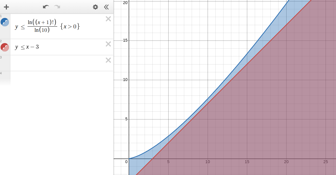
ln(10)ln((s+1)!)>d
Plotting this, we see
The linear approximation of
d≤s−3
Fits well under the entire domain.
This approximation becomes poorer as more slots are added.
When
s=70,
d≤≈100
A polynomial or piecewise approximation could provide improvement.
The original paper provides a different approximation entirely.
I have not reviewed that approximation.
When in one of the previous examples the result of
2.7180… was obtained, only 5 slots were used,
and so only two digits after the decimal place should have been expected with confidence to be correct.
Back again to thinking of the problem algorithmically:
invqr021070131041241030351021461014
Where:
iniviqiriq0=i+2=⌊(vi+qi+1)/ni⌋=(vi+qi+1)modni=nth digit of eindexdivisorvaluequotientremainder
To find the second digit, update the table such that:
This implementation seems very similar to the Algol 60 one provided in the paper.
I’m not familiar with the array syntax and semantics in Algol 60, so there may be variation there.